Bilinear Value Functions

John L. Zhou

University of California, Los Angeles

May 2026

This mini research report explores the effect of parameterizing goal-conditioned value functions with a low-rank approximation consisting of the inner (dot) product between two vectors:

where $\phi(s,a)$ and $\psi(g)$ represent “what happens next” and “where to go next,” respectively. The choice of goal representation can alternatively be conditioned on the state as well, taking the form $\psi(s,g)$ as done in Hong, Yang, & Agrawal (2022).

This inner product parameterization has a few nice properties:

1. According to the Stone-Weierstrass theorem, any continuous function $f: \mathcal S \times \mathcal S \to \mathbb R$ on a compact topological space $\mathcal S$ can be uniformly approximated by a bilinear function $\phi(s)^\top \psi(g)$. Notably, the norm $\|\phi(s) - \psi(g)\|_p$ does not enjoy these properties, regardless of the choice of $p$.
2. It enforces a low-rank structure: any matrix that can be represented as the inner product of two vectors with dimension $d$ has a rank of no more than $d$. Intuitively, high-rank matrices are undesirable because each additional linearly independent column/row carries additional information about the feature space — to prevent overfitting, we desire functions that are sparse/low-rank, so they depend on as few features as possible.

Experiments

We conduct our experiments in OGBench. We simply swap in a bilinear value function (also used in Contrastive RL) for the monolithic value function. We start with two baselines: GCIQL with DDPG+BC, which excels at short-horizon manipulation; and SAW, which is state-of-the-art in long-horizon locomotion. We perform several modifications to each method:

1. Swapping the monolithic value function network for a (late fusion) bilinear value function $Q(s,a,g) = \phi(s,a)^\top \psi(g)$.
2. Using binary cross-entropy (BCE) loss vs. mean squared error (MSE), where we simply weight the BCE loss by the expectile regression weight.
3. Clamping the target Q-value in the critic loss — between $[0,1]$ for the $[0,1]$ formulation, and between $[-1/(1-\gamma), 0]$ for the $[-1, 0]$ formulation.
4. Using early fusion with $\phi(s,a)^\top \psi(s,g)$ instead of $\phi(s,a)^\top \psi(g)$ in the bilinear value function.

To quantify performance, we measure:

• the absolute success rate (standard in OGBench)
• average time-to-completion over successful episodes

for GCIQL with DDPG+BC and SAW with GCIVL across cube-single-play, cube-single-noisy, cube-double-play, cube-double-noisy, antmaze-medium-navigate, antmaze-large-navigate, and humanoidmaze-giant-navigate.

We add the second metric due to previous observations that many successful completions (across all algorithms) in OGBench result simply from state space coverage due to a high time limit: an agent can solve most medium maze environments by simply wandering at random, and perform several incorrect placements without penalty in cube.

Main takeaways: we see massive improvements in several environments, notably cube-single-play and antmaze-medium-navigate for GCIQL and humanoidmaze-giant-navigate for SAW. We find that the choice of early vs. late fusion of goal information largely depends on the environment. For example, cube has a very simple state-goal relationship and benefits from the low-rank bottleneck imposed by late fusion, whereas puzzle demands early state-goal fusion.

Bilinear value functions with late fusion

Speed

We notice a very interesting observation in cube-single-noisy, for which GCIQL with DDPG+BC was the crème-de-la-crème — achieving 99% success in the benchmark. When swapping it for the bilinear value function, success decreased marginally (ranging around 95-97%), but the execution speed improved dramatically (around 20%).

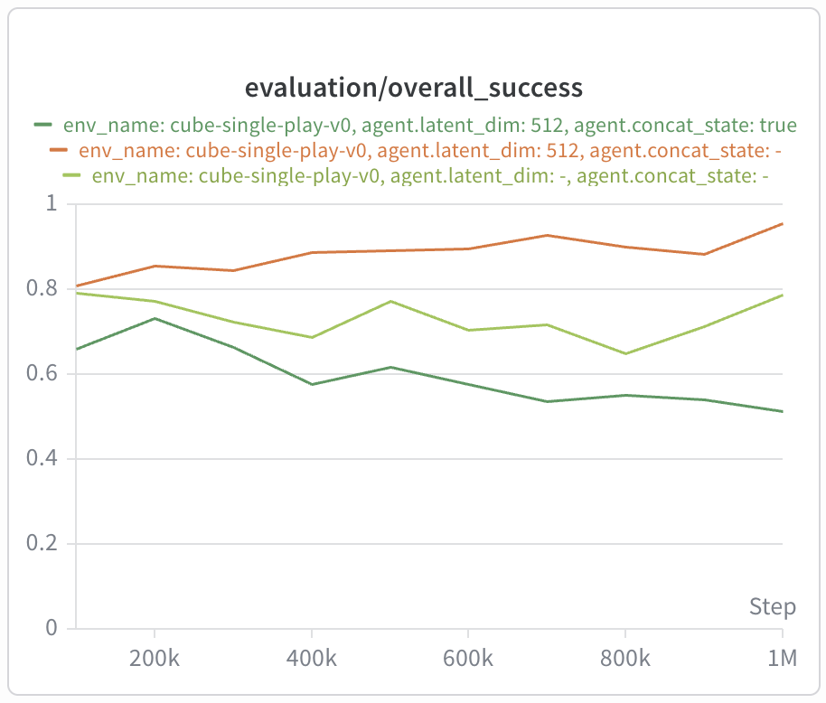
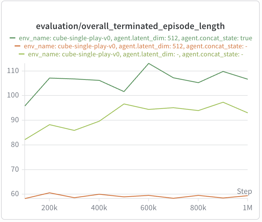
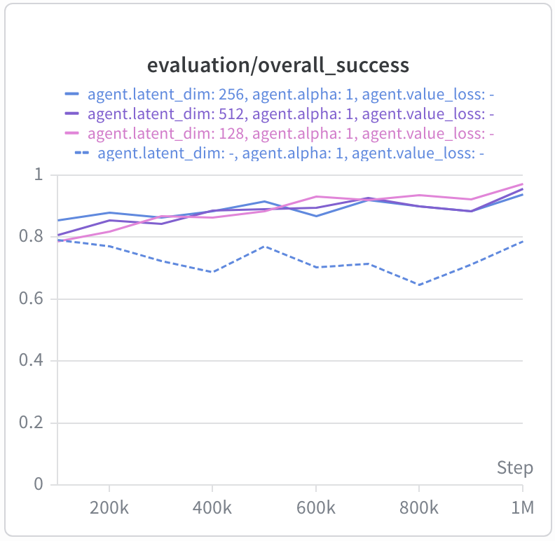
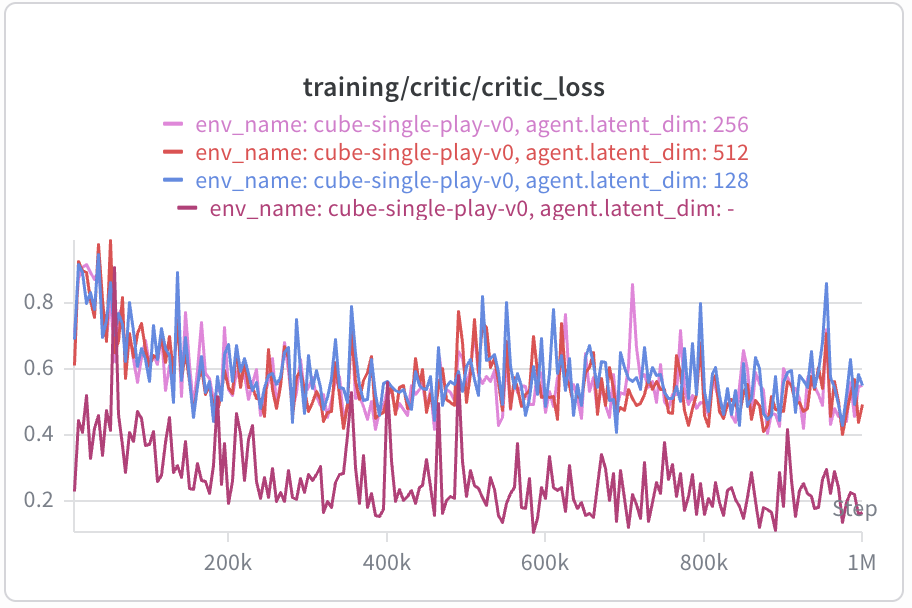
Stability

For GCIQL in cube-single-play, we often observed some amount of overfitting over the course of training (dotted line). However, the bilinear value function seems to train quite stably and improves with additional training, reaching performance comparable with cube-single-noisy!

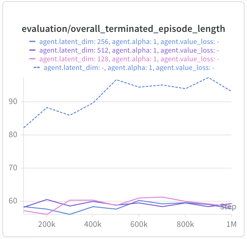
Similar to cube-single-noisy, the execution speed of the resulting policies is dramatically improved (up to 33% faster)!

Locomotion

We also observe huge improvements in locomotion, where GCIQL previously lagged behind other baselines (need to rerun to measure speed improvements).

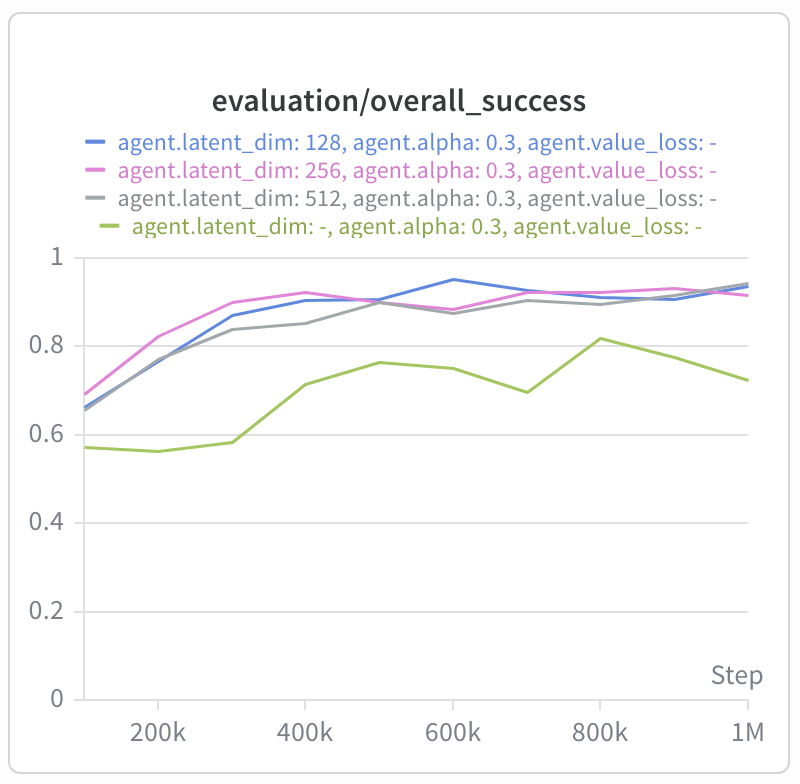
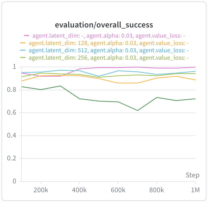
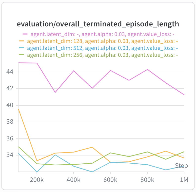
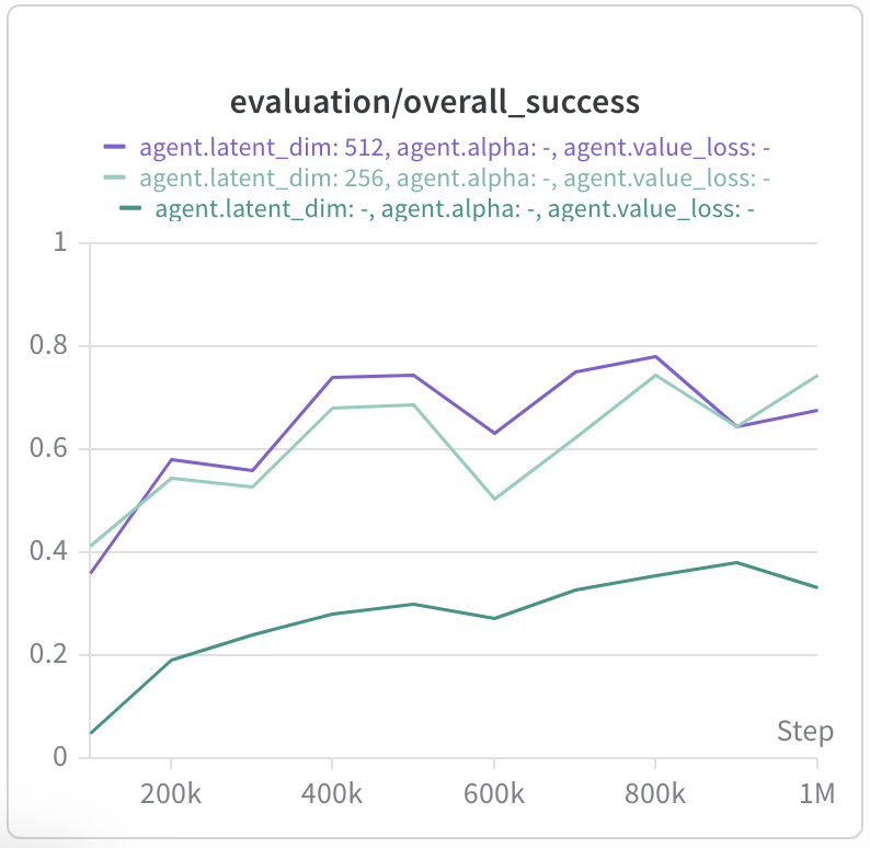
Latent dimension size

As mentioned earlier, the size of the latent dimension constrains the rank of the bilinear value function. We test ranges from $d = [16, 32, 64, 128, 256, 512]$ and generally find that values towards the higher end of the spectrum tend to do better.

Value function divergence

For cube-double-play, we observe that the value function diverges after some training, leading to collapse in performance and exploding value losses.

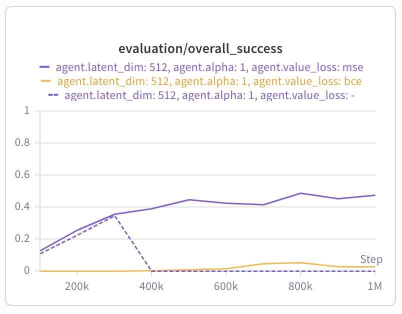
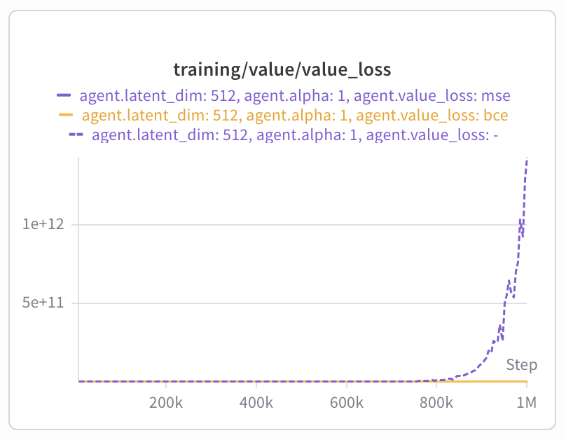
We find that this can be mitigated by clamping the Q-targets to valid ranges (3), rescuing performance. Interestingly, this does not seem to improve performance for the BCE loss.

Horizon scaling

To test the performance of the bilinear value function on long-horizon tasks, we also add it to SAW, which uses an action-free variant called GCIVL for value learning. Once again, we simply swap in the bilinear architecture. One of the main results from SAW was the ability to achieve non-trivial performance on humanoidmaze-giant, the longest-horizon task in the OGBench suite. We find that adding a bilinear value function more than doubles the performance of SAW to around 70% success rate:

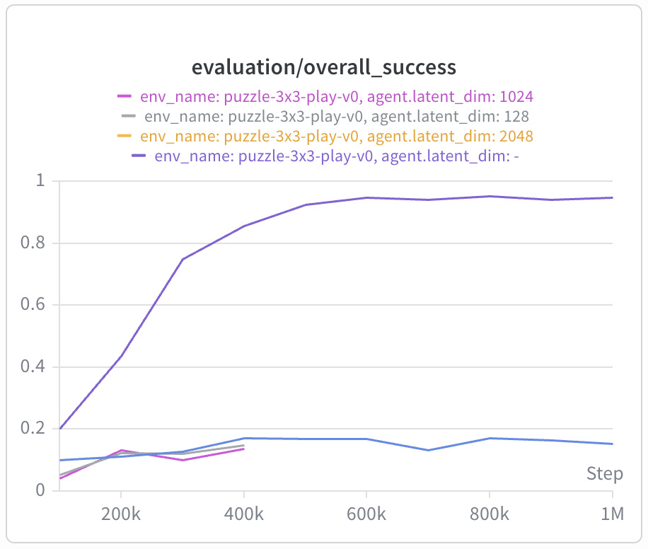
Negative results

Interestingly, the bilinear value function exhibits a significant failure mode in the puzzle environments, where GCIQL previously excelled. I tested larger latent dimension sizes (1024, 2048) to ensure that lack of expressivity was not the issue.

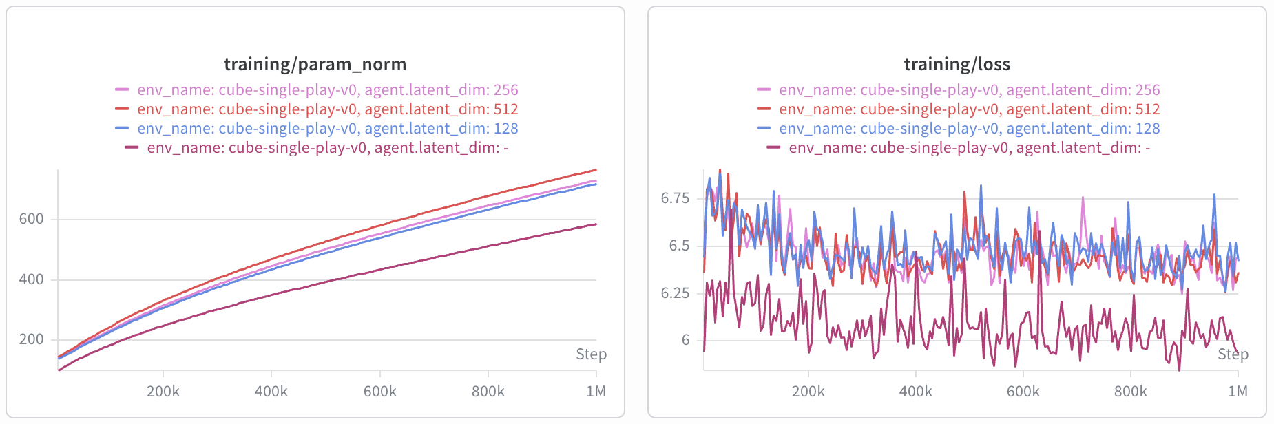
One additional interesting observation is that the parameter norms are significantly higher for BVFs, and the training loss also remains higher — the latter seems to be indicating the effects of the low-rank approximation imposed by the bilinear parameterization.

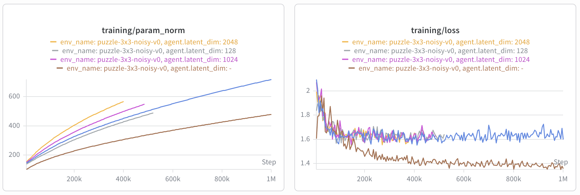
The former might just be a result of needing to learn vectors that produce a large (negative) inner product (up to $-80$ in just cube-single-play). This is also observable in the positive results, as seen below:

Hypothesis: late fusion of action with goal information makes the action gradient more noisy in DDPG+BC, since the target subgoal is highly dependent on the state-goal relationship in puzzle environments.

The puzzle consists of a two-dimensional array of buttons (e.g., a 4 × 6 grid), where pressing a button toggles the colors of the pressed button and the buttons adjacent to it.

Then, which button should be pressed next depends critically on the current state as well as the goal state, and the relationship described above may be nonlinear — only allowing a bilinear parameterization may cause underfitting as shown by the loss curve below:

On the other hand, much of the relevant information about the optimal action can be extracted only from state information in cube. For example, if the cube is not already in the gripper, it will always be the case that the correct action is to move toward the cube regardless of the goal position (this might also partially explain the degeneration in multi-cube manipulation scenarios). When the gripper contains the cube, there need only be a simple function that captures the movement from the current gripper location to the target location, which can easily be parameterized by a simple inner product.

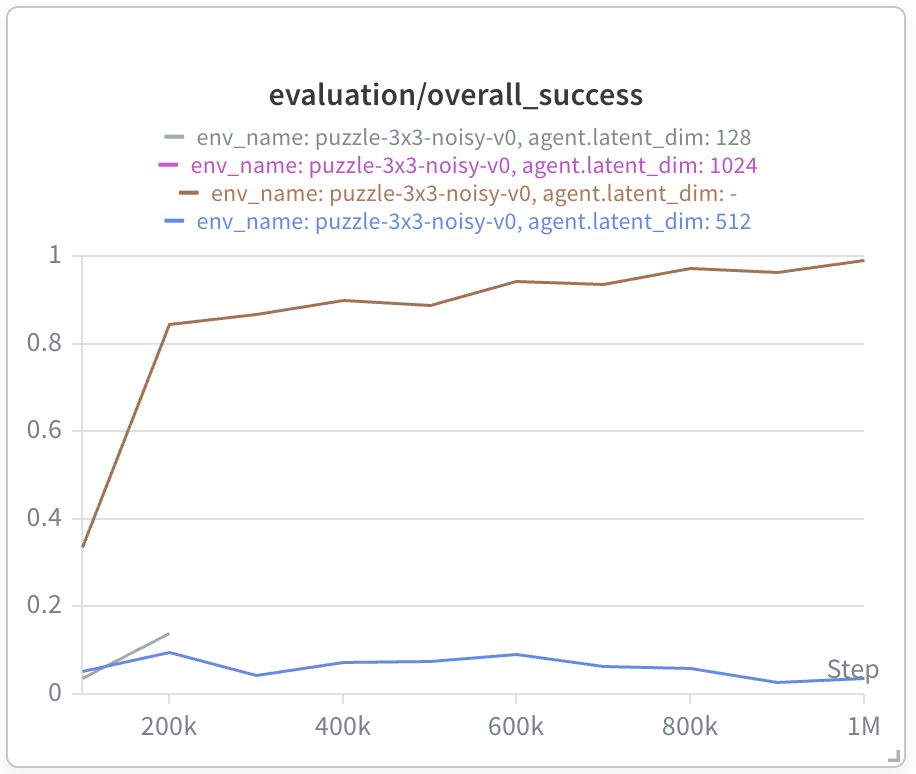
To test this hypothesis, we use the state-goal parameterization $\phi(s,a)^\top \psi(s,g)$ instead of $\phi(s,a)^\top \psi(g)$. This dramatically improves performance in puzzle (even better than the monolithic value function which is already around 95% success for both play and noisy) at the cost of significantly worse performance in cube-single.

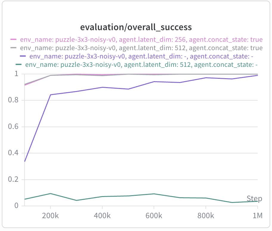
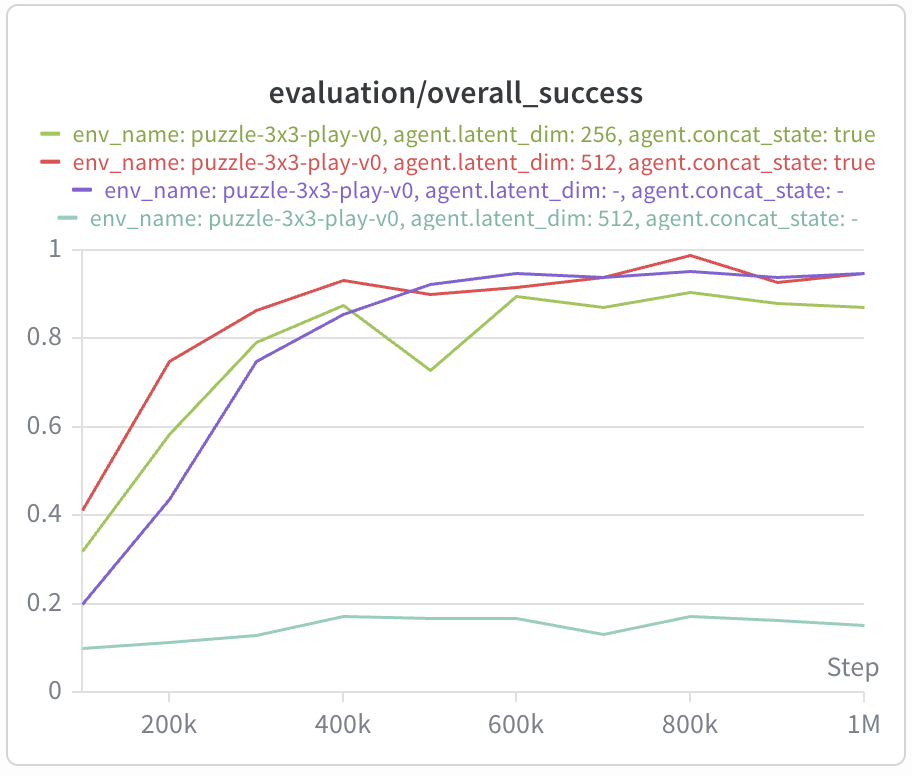
The speed of convergence and stability of BVF with concatenated state is especially outstanding — reaching stable convergence to 100% success by 200k training steps.

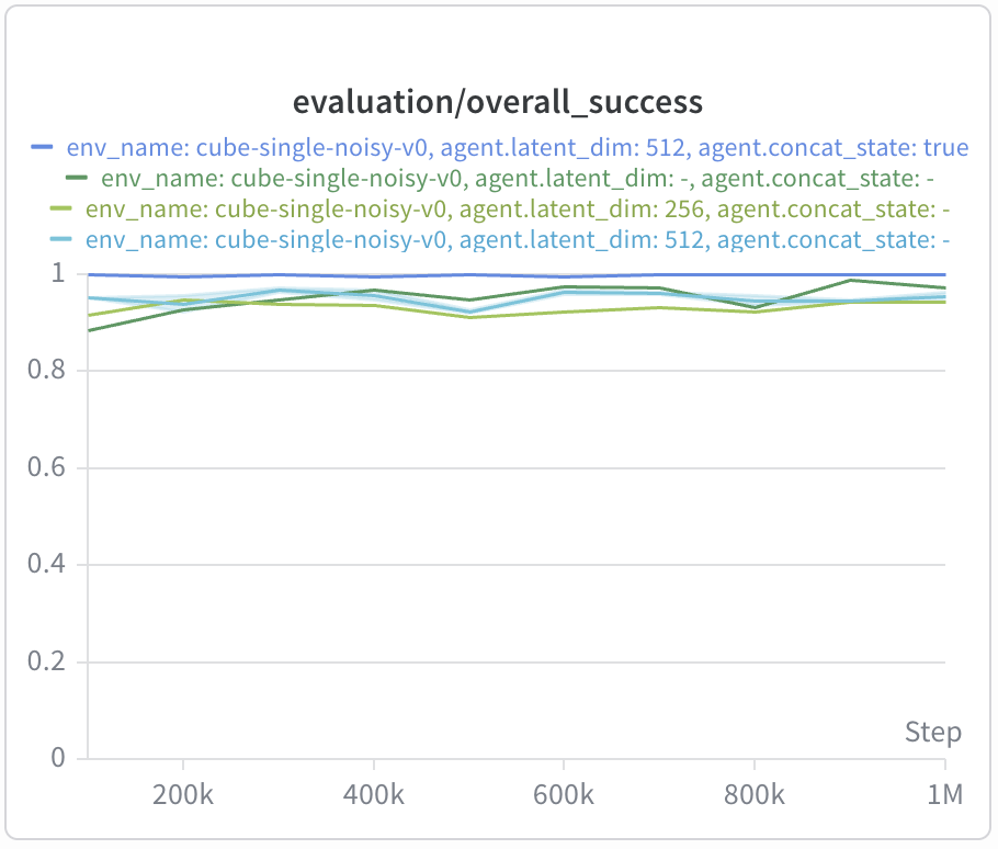
In cube-single-noisy, BVF + $\psi(s,g)$ reaches 100% success immediately and remains there during training, but is significantly slower with a similar throughput/execution speed as the original monolithic value function.

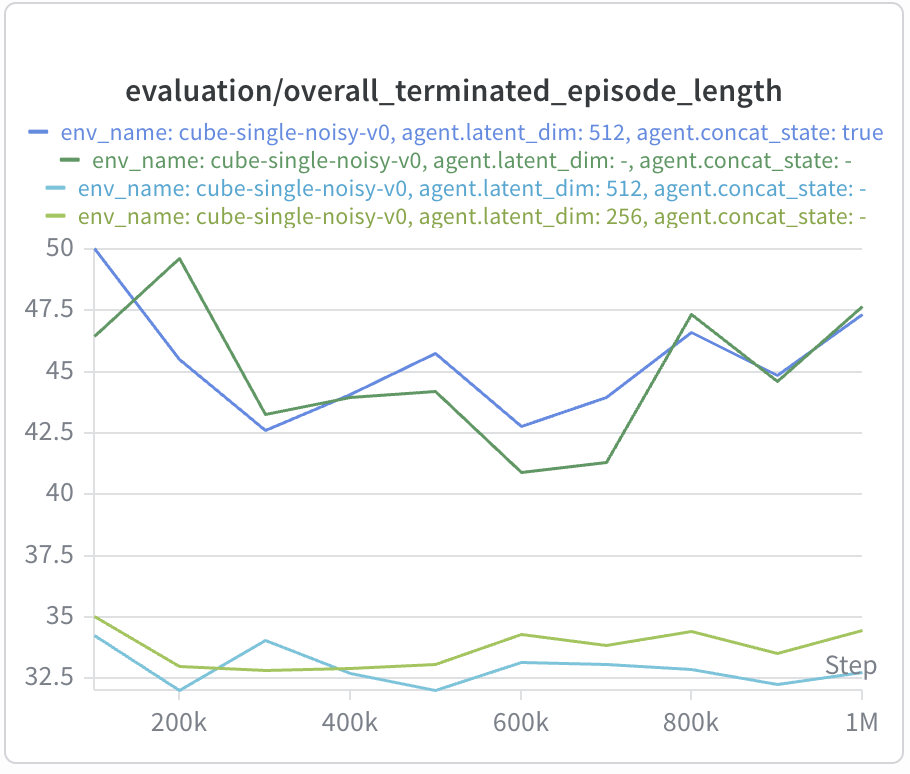
In cube-single-play, we observe both degraded performance and significantly slower execution compared to late fusion: